go-nexrad
Generating RADAR images from NEXRAD Level II data using Go.
August 25, 2017, the weekend Hurricane Harvey hit Texas I was up all hours monitoring the storm and relevant news feeds.
One tool I found was Radarscope, a superb radar app that has both desktop and mobile applications. Curious as to how weather radar imaging worked, I decided to try and figure out how to render my own weather radar images.
Here’s a sample screenshot from Radarscope of Harvey showing multiple radar products.
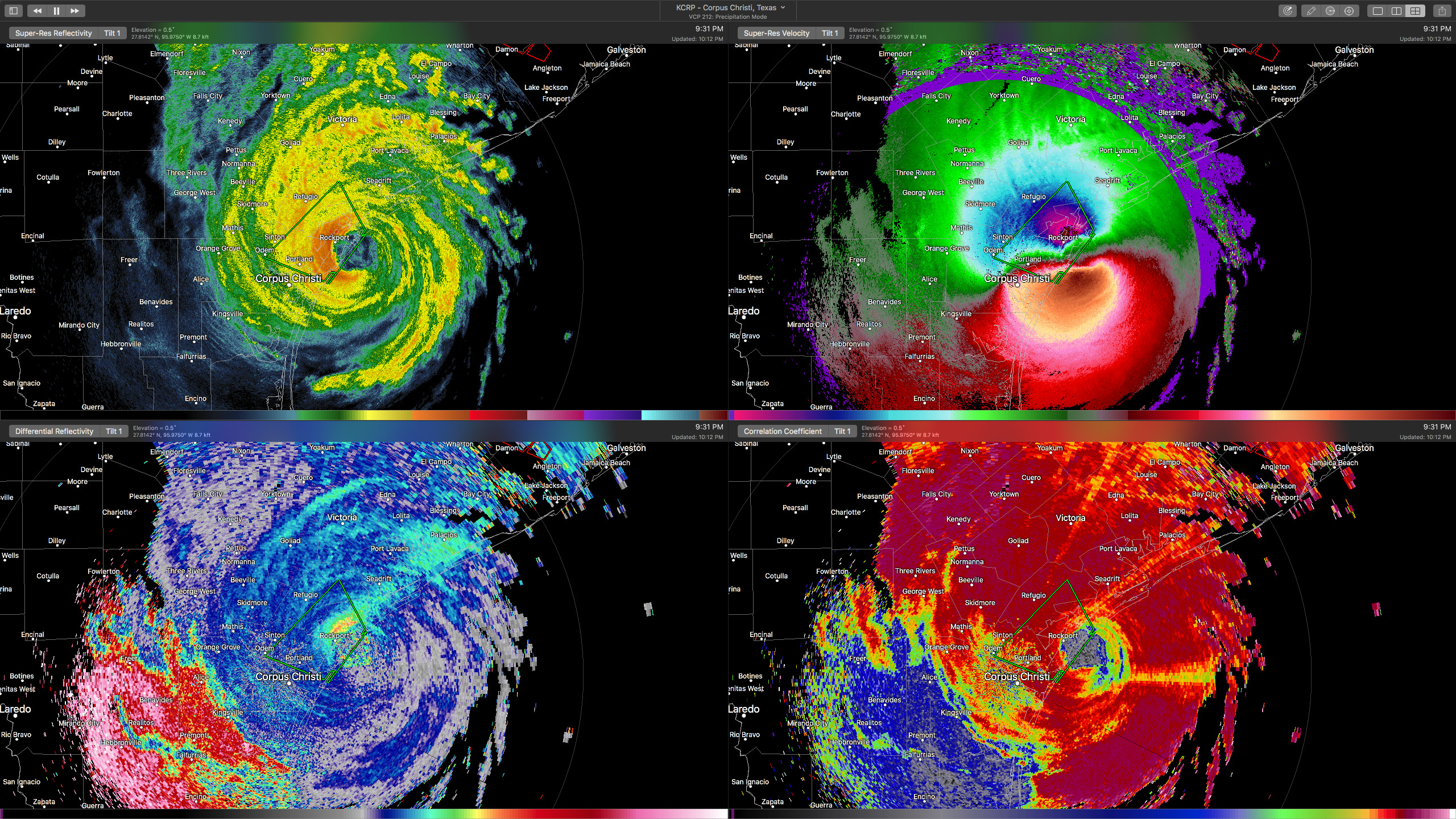
Radarscope Desktop Application
Radarscope Panes: Top left: Reflectivity, Top Right: Velocity, Bottom Left: Differential Reflectivity, Bottom Right: Correlation Coefficient
NEXRAD: Next Generation Radar
The United States runs a network of around 160 WSR-88D radars. Every few minutes (5-10ish minutes depending on the current weather situation) they scan the skys at multiple elevations and generate the radar images we’re all familiar with.
Google Streetview of NEXRAD's KGRK station in Granger, Texas outside of Round Rock
This KGRK station along with San Antonio's KEWX station provide radar coverage for Austin, Texas. If you're curious about what goes on inside a radar station, here's a tour of the KIWX Station.
Data Collection
Generating radar products happens in two phases.
- RDA (Radar Data Acquisition)
- RPG (Radar Product Generation)
RDA (Radar Data Acquisition)
The RDA phase happens when the radar is collecting data from the atmosphere.
The radar runs in two modes, clean air mode and precipitation mode. During Precipitation Mode, the radar will generate new data every 6 minutes. Clean air mode runs slightly slower, generating new data sets every 10 minutes. During that time, it will have scanned the skies at multiple elevations. The radar sends pulses out into the air, which bounce back. The strength of the bounce back determines how heavy the precipitation is. In reflectivity radar products, the heavier the objects are in the air, the more red they appear in the radar. This is why heavy rain shows in red and lighter rain typically shows in green.
For more information, check out NWS Radar: How Does the Radar Work?. It’s a solid overview of how the radar operates with some interesting technical specs.
The radars generate data and store it in an Archive II File Format (more on that format in a bit). Once the RDA phase is complete, the data is sent to the RPG unit.
RPG (Radar Product Generation)
Each Radar site hosts a computer known as the RPG unit. This computer processes the raw data and generates different products (images) for public use, which are the typical radar images you’re used to seeing.
The RPG can also run additional algorithms across multiple scans and/or elevations to create products like the Storm Total Precipitation and Vertical Integrated Liquid.
In January 2016, the NWS and Amazon teamed up to host and distribute these Level 2 data files, for free on the AWS platform. You can browse the data set using this s3 explorer. These are the files I used to generate my own radar products.
Interesting fact: NOAA had to update the color scale of their flood maps to represent how much rainfall accumulated in the Houston area.
Data Levels
There’s three levels of Radar Data. Each level relates to how much processing has to be done to the data to generate a product.
- Level I - Raw Radar Data. No processing has been done. This also doesn’t produce anything we can look at, it’s the raw binary form pulled from the radar. This is the data that I’m using for go-nexrad.
- Level II - Minimal processing, images are derived from Level I data. Includes: Reflectivity, Mean Radial Velocity, Spectrum Width, Differential Reflectivity, Correlation Coefficient and Differential Phase. These are the products that go-nexrad is replicating.
- Level III - Includes over 40 Level 3 products derived from Level I and Level II data including the base and composite reflectivity, storm relative velocity, vertical integrated liquid, echo tops and VAD wind profile.
Archive II Data Files
Now that I had found the raw data, I needed to figure out how to parse it.
I came across the ICD documentation that describe how all these systems work together and format data. Reading through the ICD FOR ARCHIVE II/USER, I was able to piece together how to parse the file format and extract the raw data out in order to render a product.
Archive II File Format
Each Archive II file contains a multi elevation scan of the sky for a certain time period. A NEXRAD radar can scan up to 20 different elevations based on the current weather situation determined by its current VCP (Volume Coverage Patterns) mode. The VCP mode is changed based on if there is precipation in the air. The VCP mode also determines if the radar should scan faster, slower, or at different elevations.
Archive II data contains multiple bzip sections which containing a Message Type.
- Message Type-2 RDA Status Data
- Message Type-3 RDA Performance/Maintenance Data
- Message Type-5 RDA Volume Coverage Pattern Data
- Message Type-13 RDA Clutter Filter Bypass Map Data
- Message Type-15 RDA Clutter Map Data
- Message Type-18 RDA Adaptation Data
- Message Type-29 Model Data Message
- Message Type-31 Digital Radar Data Generic Format - contains one (1) radial of data.
NOAA uses data from the different Message Types to update their NEXRAD Monitoring Dashboard.
Message 31 Records
Message 31 Records contain the raw data received from the Radar.
Each Message 31 Record represents a single radial of data. Think of a radial as a single radius with a degree called an azimuth. Typically a radial is 1 or 0.5 degrees. So it would take either 360 or 720 scans to complete the scan of the sky. Each radial is comprised of 1840 or so “gates”. A gate can be thought of as a single pixel of data for a point in a scan.
In the following image, each band extending from the lower right to the upperleft is a radial. Each bar within the radial is a gate.
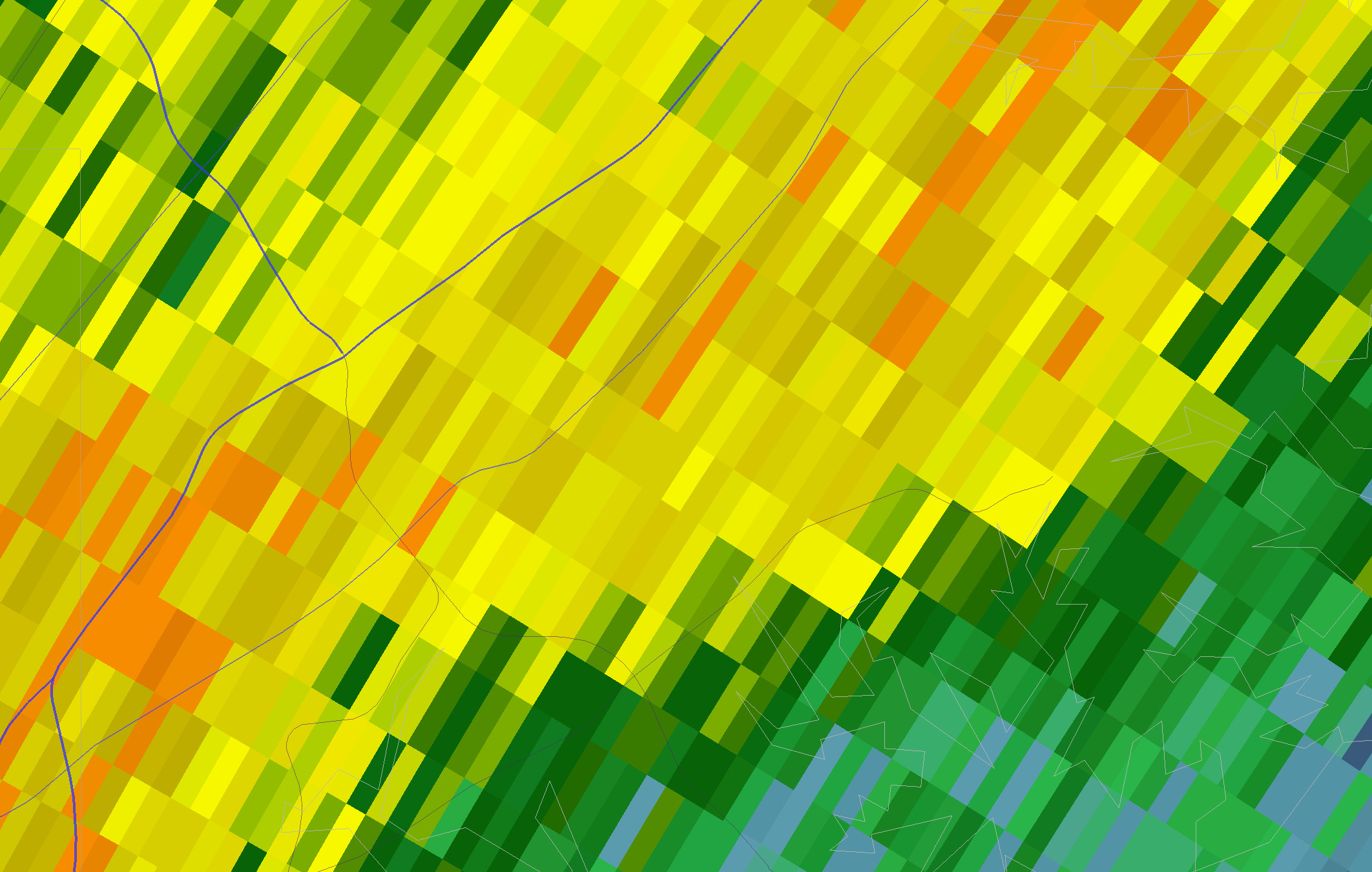
Zoomed to show Radials and Gates
Reflectivity Data
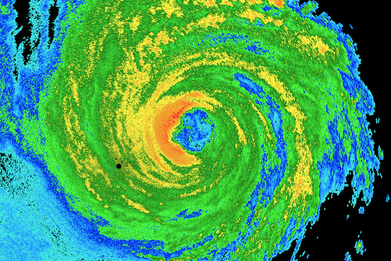
The typical green, yellow and red radar image you’re used to seeing during a storm are built from Reflectivity data, which is measured in dBZs (decibel relative to Z). The larger the dBZ the larger the precipitation (green is light rain, red is heavy rain.)
Hurricane Harvey Reflectivity
Velocity data
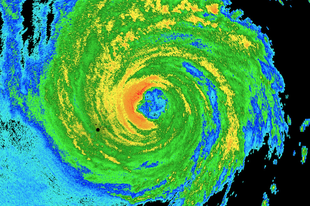
Velocity data tells you how fast a storm is moving towards or away from the radar site. Typically, in velocity products, green means things are moving towards the radar site and reds means it’s moving away. Purple means the radar timed out waiting to receive data. In the image below, you can get a sense of the counter-clockwise rotation of the storm.
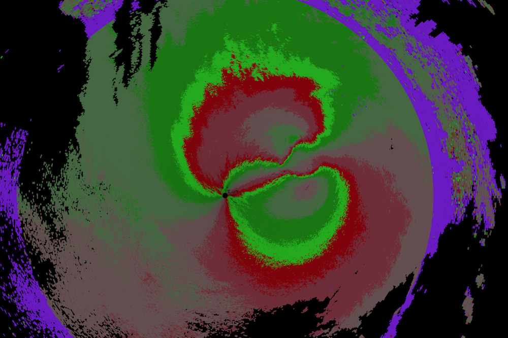
Hurricane Harvey Velocity
Rendering Notes
To render a radar image, loop through all the radials and draw each gate.
Data Point Scaling
Each data point in the Message has been scaled for easier data transfer. You have to use the offset and scale values from the record to change each 8 bit entry to a float32 that represents the actual measurement.
Gap
The radars don’t start measuring until about 0.25 km from the base station, which is why you’ll see a blank circle right around the radar in most products. You’ll need to skip out that far until you start rendering gates.
Beam Widths
Over the last 10 years or so the NWS has upgraded the resolutions for certain scans. Reflectivity and Velocity data were both updated from 1 degree resolution scans to 0.5 degree resolution scans. Depending on the data you’re rendering you’ll need to render out radials at that beam width.
Distance
Reflectivity data goes out to 400km, so you can calculate the width of each beam that way. This is also decribed in the ICD for the RDA/RPG.
Colorization
Each gate is typically represented by a certain color depending on the value. The ICD for the Product Specification contains sample colors for certain values. The document also contains information about data ranges and other details about the product (radar image) to be generated.
Concurrency
Generating a radar product from Archive II data takes a while. To process large amounts of files I ended up needing to run code concurrently. This worked out great for building animated gifs of the storm’s approach.
Usage
See the README for more additional usage info.
$ go get github.com/bwiggs/go-nexrad

$ ./nexrad-render -h
nexrad-render generates products from NEXRAD Level 2 (archive II) data files.

Usage:
nexrad-render [flags]

Flags:
-c, --color-scheme string   color scheme to use. noaa, scope, pink (default "noaa")
-d, --directory string      directory of L2 files to process
-f, --file string           archive II file to process
-h, --help                  help for nexrad-render
-l, --log-level string      log level, debug, info, warn, error (default "warn")
-o, --output string         output radar image
-p, --product string        product to produce. ex: ref, vel (default "ref")
-s, --size int32            size in pixel of the output image (default 1024)
Conclusion
This was a fascinating project to work on. I learned a lot about weather, the US Monitoring infrastructure, and RADAR technology.
It was also a great project to become more familiar with GoLang generate, file parsing, io.Readers, 2D drawing, concurrency, and flag parsing with Cobra.


